In brief: a reliable optical link needs compatible fibre, optics, connectors and a measured channel. This guide explains classes, reach, loss budgets and link verification.
Introduction: optical networks in brief
Optical networks carry information as light signals through glass fibres. A transmitter converts an electrical signal into an optical one; the receiver converts it back. The path includes fibre, connectors and splices, and in a PON also passive splitters. Glass does not conduct electricity and optical transmission is immune to electromagnetic interference. A cable may nevertheless contain metallic armour or strength members, while active electronics still require electrical safety and electromagnetic compatibility.
The core and cladding have different refractive indices and form an optical waveguide. Total internal reflection is a useful ray model; modes describe allowed field distributions, which are not confined strictly to the geometric core. Numerical aperture is NA = n₀ sin θ; it is approximately sin θ only in air where n₀ is approximately 1. Dirt and misalignment increase insertion loss and reflections.
Charles Kao and George Hockham published their landmark work on low-loss glass fibres in 1966. Fibre with loss below 20 dB/km was demonstrated in 1970. Kao received the Nobel Prize in 2009 for his contribution to optical communications. Modern telecom fibres can approach 0.2 dB/km at 1550 nm, but a real link must use the specification of its actual cable.
Applications include metropolitan and long-haul networks, buildings, data centres, subscriber access and sensing. High capacity does not remove the limits imposed by attenuation, dispersion, bending and connector condition.
FTTx terminology
| Designation | Where fibre reaches | Final section |
|---|---|---|
| FTTH | The dwelling | Optical to the subscriber terminal |
| FTTB | The building | Distribution within the building may use copper |
| FTTC | A street cabinet near subscribers | Usually copper |
| FTTN | A neighbourhood node | A non-optical section towards the subscriber |
| FTTP | Subscriber premises; an umbrella term covering FTTH/FTTB depending on context | The actual architecture must be specified |
| FTTD | The desktop/workstation | Optical to the workstation |
Passive optical networks (PON)
In a PON, an operator OLT serves multiple subscriber devices through a passive optical distribution network, ODN. ONU is a general term for the subscriber optical unit; ONT is a terminal at an end-user site, including business premises. Passive splitters need no power, but OLTs and ONTs/ONUs are active. Port capacity is shared, not a guaranteed rate for every subscriber.
| PON | Typical shared line rate: downstream / upstream |
|---|---|
| GPON (G.984) | 2.48832 / 1.24416 Gbit/s |
| EPON (802.3ah) | 1 / 1 Gbit/s |
| XG-PON (G.987) | 9.95328 / 2.48832 Gbit/s |
| XGS-PON (G.9807.1) | 9.95328 / 9.95328 Gbit/s |
| NG-PON2 (G.989) | 40 / 10 Gbit/s (TWDM, nominal aggregate) |
GPON commonly uses 1490 nm downstream and 1310 nm upstream. Class B+ allows up to 28 dB ODN loss, but this does not automatically establish 20 km reach with a 1:32 split. All splitters, joints, fibre, reserve, minimum/maximum optical levels and distance limits must be checked.
Key terms
| Term | Meaning |
|---|---|
| dB / dBm | A logarithmic power ratio: 3 dB loss is approximately half the power. dBm is absolute power relative to 1 mW. |
| Attenuation | Loss per unit length, usually dB/km at a specified wavelength. |
| Insertion loss | Power reduction introduced by a component or a complete channel. |
| Return loss / reflectance | Return loss is normally positive in dB: larger is better. Reflectance is normally negative: more negative means less reflection. |
| Dispersion | Pulse spreading; limits the supported combination of rate and distance. |
| Bandwidth | Modal bandwidth in MHz·km; not directly a data rate in Gbit/s. |
| Mode | An allowed spatial field distribution in the waveguide. |
| Loss budget | Permitted loss for a particular application, distinct from an arbitrary engineering reserve. |
1. Basic differences
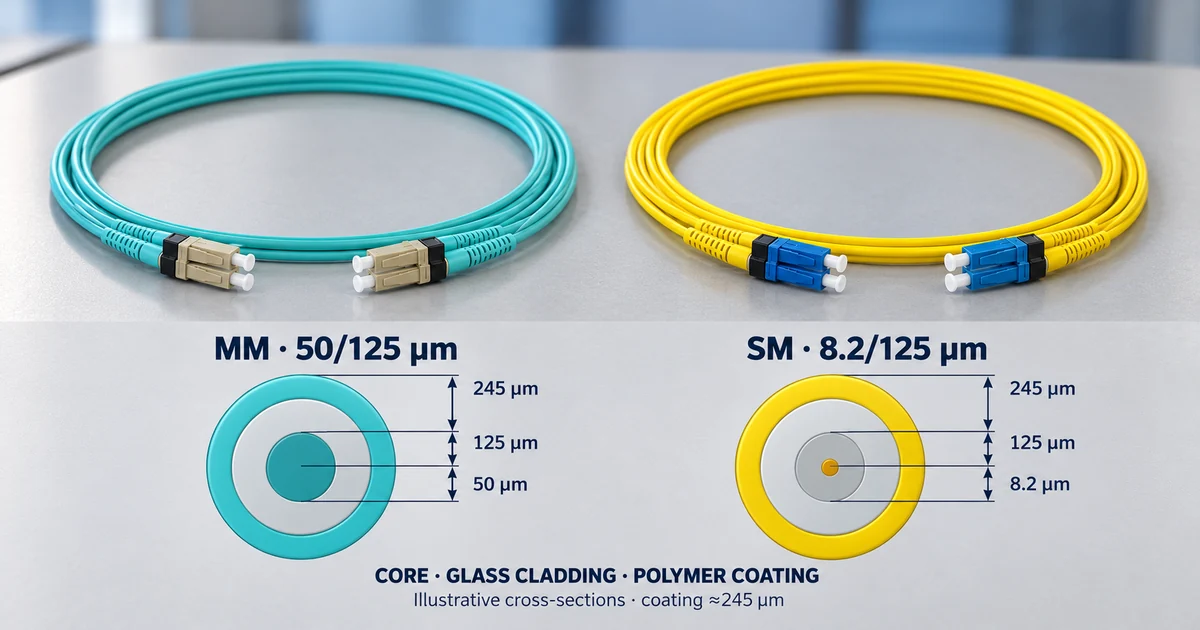
For the cabling considered here, multimode fibre is 62.5/125 µm for OM1 or 50/125 µm for OM2–OM5. The first number is core diameter and the second is glass cladding diameter. “9/125” is a practical single-mode designation rather than an exact universal dimension. Mode field diameter (MFD) is a separate wavelength-dependent parameter and need not equal the geometric core diameter.
| Parameter | Multimode (MM) | Single-mode (SM) |
|---|---|---|
| Core | OM1: 62.5 µm; OM2–OM5: 50 µm | ~9 µm; MFD ≠ core |
| Cladding | 125 µm | 125 µm |
| Propagation | many modes (light paths) | one mode |
| Wavelengths | 850 nm (and 953 nm for OM5), 1300 nm | 1310 nm and 1550 nm |
| Transmitter | LED or VCSEL laser (850 nm), 1300 nm | laser (Fabry-Pérot, DFB and others) |
| Distance limit | modal dispersion | chromatic and polarisation mode dispersion, attenuation |
| Typical use | building, campus, data centre | between buildings, metro and long-haul routes |
| Jacket colour (TIA-598) | orange (OM1, OM2), aqua (OM3, OM4), lime (OM5) | yellow |
Multimode links commonly use 850 or approximately 1300 nm. Single-mode systems widely use 1310 and 1550 nm, with additional bands in PON and other systems. OM5 is wideband multimode fibre intended for the 850–953 nm region. Intermodal dispersion spreads pulses in multimode fibre. Single-mode fibre avoids intermodal dispersion, but chromatic and polarisation mode dispersion remain. The application, not distance alone, determines the choice.
2. Multimode fibre: classes OM1–OM5
OM1 and OM2 are legacy classes. New multimode cabling normally considers OM3, OM4 or OM5 according to the application. OFL is overfilled-launch bandwidth; EMB is effective modal bandwidth under conditions relevant to laser launch. These measures are not interchangeable.
| OM | µm | OFL 850 nm | EMB 850 nm |
|---|---|---|---|
| OM1 | 62.5/125 | 200 | — |
| OM2 | 50/125 | 500 | — |
| OM3 | 50/125 | 1500 | 2000 |
| OM4 | 50/125 | 3500 | 4700 |
| OM5 | 50/125 | 3500 | 4700 |
All bandwidth figures in the table are in MHz·km. OFL at 1300 nm is 500 for all five classes. OM5 has OFL 1850 and EMB 2470 at 953 nm. OM5 does not automatically extend a standard single-wavelength 850 nm link beyond OM4; its advantage concerns compatible multiwavelength solutions. Colour is a guide, not proof of the fibre class: check markings and documentation.
The light distribution launched by a test source affects multimode loss results. Encircled-flux conditions in IEC 61280-4-1/TIA-526-14 limit this uncertainty. The test method, adapters and reference cords must suit the fibre under test.
3. Single-mode fibre: OS1, OS2 and ITU-T G.652/G.657
OS1/OS1a and OS2 are single-mode cabling categories; G.652/G.657 describe fibre characteristics. They are different classification systems. OS2 does not mean “outdoor only”: suitable indoor cable constructions also exist. Technical guidance lists a maximum of 1.0 dB/km for OS1a and 0.4 dB/km for OS2 at the specified wavelengths; exact requirements depend on the applicable edition and product.
| Fibre | Practical significance |
|---|---|
| G.652.D | Standard single-mode fibre with zero dispersion near 1310 nm and a low water peak. |
| G.653 | Dispersion shifted towards 1550 nm; specialised applications. |
| G.654 | Cut-off-shifted fibres for particular long-haul systems. |
| G.655 | Non-zero dispersion-shifted fibre for multiwavelength systems. |
| G.657 | Improved macrobend performance; check the category and the actual cable. |
The fifth edition of G.657, published in 2024, merges category B2 into A2. The current description uses A1, A2 and B3. Category A aligns with G.652.D requirements; B3 targets tighter bending and compatibility must be assessed for the system. The 10, 7.5 and 5 mm values describe category-specific bend test conditions. They are not universal installation bend radii for finished cables: follow the cable manufacturer’s radius, tensile and installation limits.
4. Attenuation and loss budget
| Fibre | Wavelength | Illustrative coefficients for a teaching calculation |
|---|---|---|
| Multimode (50/125, 62.5/125) | 850 nm | 3.5 dB/km |
| Multimode | 1300 nm | 1.5 dB/km |
| Single-mode, indoor | 1310 and 1550 nm | 1.0 dB/km |
| Single-mode, outdoor | 1310 and 1550 nm | 0.5 dB/km |
This table uses illustrative conservative coefficients, not universal limits for every indoor or outdoor cable. OS2 is often specified at a maximum of 0.4 dB/km at the relevant wavelengths; use the actual cable datasheet. Add connector, splice, splitter and filter losses, plus an explicit reserve, to α × L. Minimum transmit power minus receiver sensitivity is an optical power budget; permitted channel insertion loss may impose further constraints.
L = α × length + Σ connectors + Σ splices + Σ splitters/filters + reserve
| Application | Wavelength | Permitted channel loss |
|---|---|---|
| 1000BASE-SX on OM1 / OM2 / OM3 / OM4 | 850 nm | 2.6 / 3.6 / 4.5 / 4.8 dB |
| 1000BASE-LX (multimode) | 1300 nm | 2.3 dB |
| 1000BASE-LX (single-mode) | 1310 nm | 4.5 dB |
| 10GBASE-SR on OM1 / OM2 / OM3 / OM4 | 850 nm | 2.4 / 2.3 / 2.6 / 2.9 dB |
| 10GBASE-LRM | 1300 nm | 1.9 dB |
| 10GBASE-LR | 1310 nm | 6.2 dB |
| 10GBASE-ER | 1550 nm | 11.0 dB |
For 10GBASE-SR on OM4/OM5 at 400 m, permitted channel loss is 2.9 dB. The 4.5/4.8 dB 1000BASE-SX values for OM3/OM4 are planning figures for extended profiles, not universal requirements of the original IEEE standard. Low loss alone does not prove a link will work: also check maximum reach, dispersion, reflections, receiver overload and the actual module specification.
Example 1 (illustrative, calculated from the limits above)
A 1000BASE-SX link over OM3, 400 m, two connector pairs, no splices. Attenuation: 0.4 km × 3.5 dB/km = 1.4 dB. Connectors: 2 × 0.75 = 1.5 dB. Total 2.9 dB against a permitted 4.5 dB: a margin of 1.6 dB.
Example 2 (illustrative)
A 10GBASE-LR link over outdoor single-mode fibre, 8 km, two connector pairs and four splices. Attenuation: 8 × 0.5 = 4.0 dB. Connectors: 2 × 0.75 = 1.5 dB. Splices: 4 × 0.3 = 1.2 dB. Total 6.7 dB against a permitted 6.2 dB: it does not fit in the worst case. With typical manufacturer values (for example 0.33 dB/km and less than 0.3 dB per connector and 0.1 dB per splice) the loss is much smaller, which is why a real link is measured rather than judged by limit values alone.
5. Which fibre for which Ethernet
| Application | Fibre | Indicative channel reach |
|---|---|---|
| 1000BASE-SX | OM1 / OM2 | 275 m / 550 m |
| 1000BASE-LX | MM / SM | 550 m / 5 km |
| 1000BASE-LX10 | MM / SM | 550 m / 10 km |
| 10GBASE-SR | OM1 / OM2 / OM3 / OM4 / OM5 | 33 / 82 / 300 / 400 / 400 m |
| 10GBASE-LRM | MM | 220 m |
| 10GBASE-LR | SM | 10 km |
| 10GBASE-ER | SM | 40 km (engineered link >30 km) |
| 40GBASE-SR4 | OM3 / OM4 | 100 / 150 m |
| 100GBASE-SR4 | OM3 / OM4 | 70 / 100 m |
The table summarises specific applications, not every optic operating at that rate. The 275 m 1000BASE-SX figure assumes OM1 with 200 MHz·km; older 160 MHz·km fibre has a different limit. Extended reaches around 1 km on OM3/OM4 depend on the profile and vendor, not a universal guarantee from the original standard. A 10 km 1000BASE-LX/LH product specification does not change the basic 5 km 1000BASE-LX reach. LX10 is a separate application.
10GBASE-LRM normally supports up to 220 m on specified multimode fibre. A vendor’s 300 m single-mode capability is product-specific. 40GBASE-SR4 supports 100 m on OM3 and 150 m on OM4; 100GBASE-SR4 supports 70 and 100 m respectively. Do not apply these figures to SR10, BiDi or SWDM. Check the exact modules, fibre, lane count, length and loss budget.
6. Mixing fibres and modules
Matching connector shapes do not establish optical compatibility. Rate, optical application, wavelength, fibre type and power limits must match; BiDi requires a correctly paired transmitter/receiver wavelength combination.
A transition between 50 and 62.5 µm, or between multimode and single-mode fibre, has loss dependent on direction, launch, mode field and components. There is no universal “17–20 dB in both directions”. Low insertion loss can coexist with unacceptable dispersion. Different 50/125 µm classes may sometimes be combined when compatibility is demonstrated, but performance is limited by the weaker section.
A mode-conditioning patch cord (MCP) launches light off-centre into multimode fibre for specified legacy applications. A manufacturer may require it for particular 1000BASE-LX/LH, LX4 or LRM modules on OM1/OM2. The correct type is installed at both ends on the correct transmit leg. It is not added arbitrarily to 850 nm SX/SR or OM3/OM4/OM5 links, and it is not a universal MM↔SM converter.
An ordinary passive adapter changes the mechanical connection; it does not make incompatible optical systems compatible. Where a transition is needed, an active optical-electrical-optical solution such as a media converter or switch with an appropriate optic on each side is practical.
7. Connectors and end face
| Connector | Ferrule | Coupling | Interface series |
|---|---|---|---|
| LC | 1.25 mm | Latch | IEC 61754-20 |
| SC | 2.5 mm | Push-pull | IEC 61754-4 |
| ST | 2.5 mm | Bayonet | IEC 61754-2 |
| FC | 2.5 mm | Threaded | IEC 61754-13 |
| MPO | Rectangular MT | Push-pull | IEC 61754-7 |
LC uses a 1.25 mm ferrule; SC, ST and FC use 2.5 mm ferrules. MPO is a multifibre interface with a rectangular MT ferrule. Polarity, fibre count and guide-pin configuration must also match. Connector shape alone does not establish SM/MM type or application.
APC commonly uses an 8° end-face angle and a green housing; UPC has a different polish. APC and UPC must not be mated: loss, reflections and damage can result. Colour is only a guide. The cleaning sequence is “inspect → clean if needed → inspect again”. Use an appropriate video probe after checking optical power; never look directly into a fibre.
8. Splicing
Fusion and mechanical splicing are used for both single-mode and multimode fibre. Fusion is widespread for permanent links; mechanical products may be temporary or permanent according to their specification. The choice depends on the environment, tools and permitted loss.
- Prepare the cable and service slack; fit the splice protector before splicing.
- Remove buffer and coating as required by the construction. Not every fibre has a 900 µm buffer.
- Clean with approved materials and cleave precisely using the appropriate tool. Do not touch the cleaved end face.
- Align and fuse using a programme suitable for the fibres and a calibrated instrument.
- Review the splicer estimate. It is an estimate, not an independent measurement. Prepare a defective splice again.
- Protect and store the splice in its tray without exceeding bend or tension limits.
Manufacturers demonstrate fusion losses below 0.05 dB under good conditions, but this is not guaranteed for every joint. Fibres and field conditions differ. A 0.75 dB connector-pair allowance and a 0.3 dB splice allowance can serve as conservative teaching assumptions; acceptance limits belong to the particular channel. Do not create an arbitrary MM–SM transition by fusion splicing.
9. Testing and verification
- An OLTS — a light source and power meter — measures end-to-end loss at the relevant wavelengths with the correct reference procedure.
- An OTDR locates events, splices and faults. Use suitable launch and receive fibres, settings and measurements from both ends when evaluating splices.
- Different backscatter coefficients can produce an apparent negative-loss event, or “gainer”, on an OTDR trace. Averaging measurements of the same event in both directions reduces this error; a splice does not amplify light.
- OLTS and OTDR complement one another. End-face video inspection, continuity and polarity checks also matter. Record method, length, wavelength, direction, reference, losses and acceptance criteria.
10. Which document is for what
| Document | Subject |
|---|---|
| ITU-T G.652, G.657, G.653–G.656 | Types of single-mode fibre |
| IEC 60793-2-50 (single-mode), IEC 60793-2-10 (multimode) | Product specifications of the fibre |
| TIA-492AAAx (MM), TIA-492CAAx (SM) | Fibre specifications under TIA |
| ISO/IEC 11801, TIA-568.3 | Cabling and components, OM/OS classes, loss limits |
| TIA-598 | Jacket colours |
| IEC 61754 (series) | Connector geometry |
| IEC 61300, IEC 61753-1 | Tests and performance grades of connectors |
| IEC 61280-4-1 / TIA-526-14, TIA-526-7 | Loss measurement (multimode and single-mode) |
| IEEE 802.3 (clauses 38, 52, 59, 68 and others) | Which fibre and distance each Ethernet standard allows |
11. Typical mistakes
- Module and fibre of different type (an SM module on MM fibre or the reverse).
- A mode-conditioning patch cord on OM3 or on an 850 nm link.
- A dirty or scratched connector: the most common cause of a bad link.
- A poor cleave before fusion.
- A bend radius below the permitted one (especially with older fibre, not G.657).
- A budget calculated only with typical values and not checked by measurement.
- Connectors of different type in one link (APC to UPC).
12. Safety
Active optics can emit invisible infrared light. Do not look into a fibre or connector. Establish whether optical power is present before inspection and follow the equipment procedures. An appropriate video probe is preferable to direct viewing through an optical eyepiece. Collect glass shards in a dedicated closed container. The IEC 60825 series addresses laser safety.
Note on reliability
The material was checked against publicly available ITU-T recommendations, manufacturer data and TIA FOTC guidance. Complete paid IEC/ISO/TIA texts are not represented as directly reviewed. Figures for particular modules are not universal fibre properties. Real links require the applicable edition, exact component documentation and measurement.
Sources
- ITU-T G.652 (2024)
- ITU-T G.657 (2024)
- TIA FOTC — optical fibre types
- Cisco — OM4 / OM5, OFL / EMB
- Corning — OM5 bandwidth
- TIA FOTC — 10GBASE-SR
- TIA FOTC — 1000BASE-SX
- TIA FOTC — 1000BASE-LX
- Cisco — 10G optical modules
- Cisco — 40G optical modules
- Cisco — 100G optical modules
- Cisco — mode-conditioning patch cords
- CommScope — OS1a / OS2
- Corning — optical definitions
- Corning — fusion splicing AN103
- Fluke Networks — OLTS / OTDR
- Fluke Networks — fibre testing and inspection
- ITU-T — GPON physical layer
- ITU-T — XGS-PON
- ITU-T — NG-PON2
- Nobel Prize — Charles Kao lecture